The first week of Google Summer of Code has ended, and so it's time for a recap post!

The main topic this week was PartDesign Mirrored, a fairly self-explanatory feature, with a show-stopping bug explained in FreeCAD issue 3006.

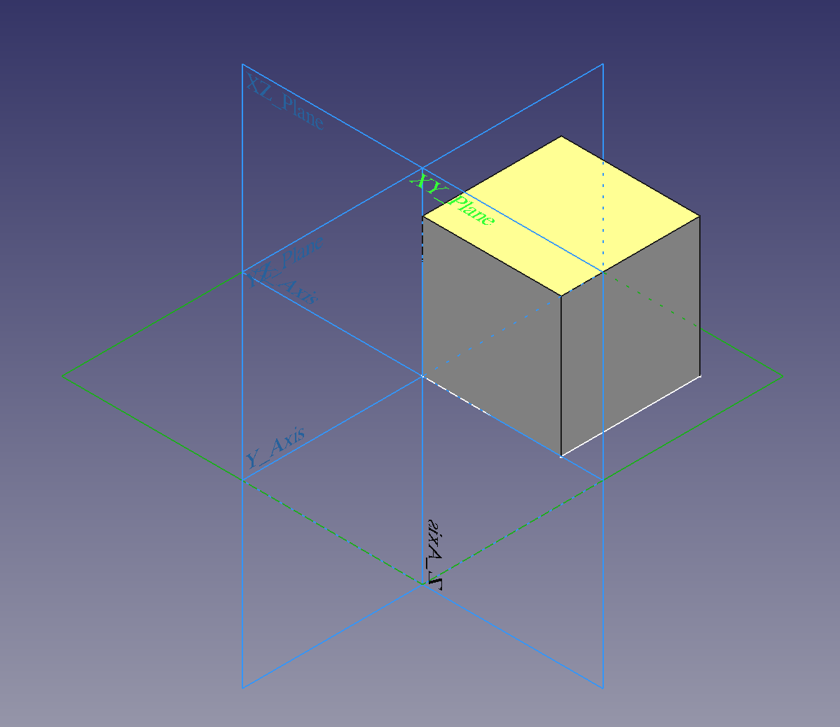
Figure 1. The base of my PartDesign Mirrored experiments.

In this picture, we have a simple 1 mm square sketch (pictured in white) attached to the \(xy\)-plane. One corner is at the origin, and the sketch is the base for a Pad feature 1 mm high. Length is handled internally as mm by FreeCAD, so this "unit cube" serves as a useful basis for testing behavior. A useful alteration involves displacing this cube, say, 1 mm up the \(y\)-axis. This constructs a case where mirroring not all mirrorings should succeed, but we'll get into that later.

Let's turn now to the bug itself, depicted in figure 2. The unit cube is supposed to be mirrored about its vertical sketch axis (the \(y\)-axis, pictured running off to the top right.) Obviously, it's not, and the failure is helpfully represented in red.

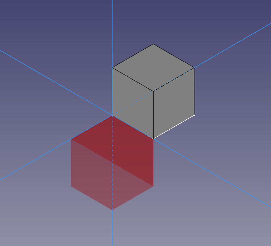
Figure 2. FreeCAD bug 3006 in action.

Note that the body diagonal of the mirrored part should run from the origin to \((-1, 1, 1)\). Instead, it's going to \((1, -1, -1)\), in the opposite direction.

Well, this was my first really serious bug to tackle for the summer. I chose this as a way to really dive in, since it directly involves Open CASCADE, the open source C++ geometry kernel at the heart of FreeCAD.

However, my programming background is chiefly with Python (as well as JavaScript and Lua), all interpreted languages. One nicety of that sort of language is that it can be very quick to debug and examine behavior using the interpreter. There is a Python debugger, pdb, but I rarely needed to use it for my mostly personal-sized projects. Even then, it's quite straightforward to use since you're already in an interpreter-native environment.

C++ is a very different beast. In this case, stepping through the code with a debugger was my only choice. I use Neovim as my IDE, though, so I wanted a way to combine the power of my text editor with my debugger. So, I found and set up LLDB.nvim, an LLDB frontend, with an event-based, non-blocking UI, session-saving, and "... takes advantage of Neovim's job API to spawn a separate process and communicates with the Neovim process using RPC calls."

Pretty nice. Anyway, I was able to step through the code and see exactly what was flying around, just like I wanted.

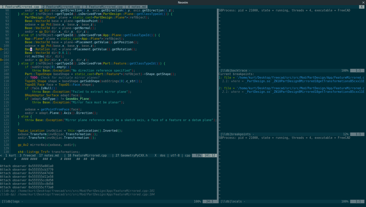
Figure 3. Neovim in an LLDB debug session.

So, what was the problem? Hah! Not so simple. Turns out there are at least four bugs here!!

First, the algorithm which first checks if the mirrored shapes are adjacent and thus, can be fused, was broken.

Once this failed, FreeCAD then attempts to generate a mesh from the shape, and then converts a generalized transformation object representing the mirroring into a matrix to put the mesh in the correct place. It turns out that in Open CASCADE 7.0.0, the gp_Trsf API was changed so that gp_Trsf::VectorialPart() returns a 3x3 matrix including the scale factor. The previous behavior was to return the homogeneous part of the transformation which does not include the scale factor, and the FreeCAD algorithm for constructing the 4x4 matrix for the mesh included multiplying every term by a scale factor. In other words, the scale factor multiplication was happening twice. The scale factor I had observed in the debugger was -1, so this perfectly explained the inverted positioning of the failure result!

The third bug, of a much more minor nature, involved a a classic "failure... success!" message displayed in the event of a mirroring failure, and was easier to fix.

The fourth, though, was a bit trickier! It only appeared when fixing the mesh placement.

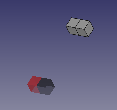
Figure 4. A strange, new mirroring bug.

This one was diagnosed by ickby, my mentor for this project. It turns out the failure meshes' faces were getting constructed inside out, and so the material's color was not considered "illuminated".

The three of us considered a few different options to get around this. One way would be to use Coin3D, FreeCAD's scene graph library, and change the material properties to define something that looked the same, illuminated or not. Another is to essentially duplicate each face with the second instance having an inverted normal, so that you're guaranteed to have an outward-facing face.

The fix ended up being much simpler than that! It was possible to simply change the vertex ordering. Originally, it was set to COUNTERCLOCKWISE. However, in figure 4, you can see that simply changing it to CLOCKWISE would not be an obvious fix. Abdullah also fixed this one, presumably by checking the docs for that option and finding that there was an "option C", UNKNOWN. That did the trick!

So now, PartDesign Mirrored is fixed and ready. Not a bad start for the summer!

It's been almost a year since my last post, which just so happened to be about FreeCAD as well. It's been a busy year: I've been studying machine design, robotics; partial differential equations in general, and heat and mass transfer in particular. I've also been studying the source code of FreeCAD while honing my sysadmin skills by helping maintain project infrastructure. My hard work has paid off, and my Google Summer of Code project proposal was accepted! I'm going to be working on improving the parametric part design workbench and writing test code to make the module more robust for future development.

As a result, I've decided to publish my daily log here. I'll be posting weekly summaries once the coding period begins on May 30, as well as more in-depth ad hoc blogging on interesting developments over the summer. My goal is to both document my project and to produce a useful reference for other developers wanting to get started contributing to FreeCAD.

The rest of May is part of the Community Bonding Period, and so I'll ramp up to full speed with an introductory series of posts. Here are a few rough-draft titles to highlight my planned topics:

• Neovim as an IDE:

  1. Building your base, or practically pluginless

  2. What makes an IDE? An overview of features

  3. Unix as an IDE, or knowing your tools

  4. Neovim with Python 2 and 3

  5. Neovim with C++

  6. Asynchronous autobuilding with Neovim

• Distributed compilation with distcc

• Speaking source code: how to fix your first FreeCAD bug

• Contributing to open source communities (and FreeCAD in particular)

FreeCAD is a multi-platform (Windows, Mac, Linux) open source parametric 3D CAD modeler, and can read and write many open file formats.

An explanation of the many virtues of open source software can be found at Open Source for America and elsewhere. To quote OSFA,

The Open Source model harnesses the power of distributed peer review and transparency to create high-quality, secure and easily integrated software at an accelerated pace and lower cost.

Commerical-grade CAD software, while incredibly useful, has several downsides including being locked behind 4 or 5 digit licensing costs, and its use in amateur projects or the developing world is often facilitated by piracy. FreeCAD, on the other hand, is free as in beer and free as in freedom, although it is currently under development. However, one of the benefits of the open source model is the ease with which interested people can contribute to the project and make better tools for all mankind.

While using FreeCAD, I noticed a few typos in the menus; although my first contribution to the project wasn't too significant, I documented the process of getting a development environment set up on my Ubuntu 16.04 desktop so that others could follow the same steps and begin contributing.

1. Pull down a copy of the code. (If you don't have a copy of git, run sudo apt-get install git.)

git clone https://github.com/FreeCAD/FreeCAD.git freecad-code
mkdir freecad-build

2. Install all dependencies.

sudo apt-get install build-essential cmake python python-matplotlib libtool libcoin80-dev \
  libsoqt4-dev libxerces-c-dev libboost-dev libboost-filesystem-dev libboost-regex-dev  \
  libboost-program-options-dev libboost-signals-dev libboost-thread-dev libboost-python-dev \
  libqt4-dev libqt4-opengl-dev qt4-dev-tools python-dev python-pyside pyside-tools 'liboce*-dev' \
  oce-draw libeigen3-dev libqtwebkit-dev libshiboken-dev libpyside-dev libode-dev swig libzipios++-dev \
  libfreetype6 libfreetype6-dev

# Install optional packages
sudo apt-get install libsimage-dev checkinstall python-pivy python-qt4 doxygen \
  libcoin80-doc libspnav-dev

3. Move into build folder, make and compile the software. Use the -j $(nproc) flag to use all N of your CPU cores when compiling; some recommend using N + 1 CPU cores, which can be done by instead running make -j$(( $(nproc) + 1 )) .. Don't forget the period at the end of the make command, which tells it to put the compiled software in the current freecad-build directory; it's good to keep the source code and build directories separate.

cd freecad-build
cmake ../freecad-code
make -j$(nproc) .

4. Fix Ubuntu 64-bit issue. If you are using a 64-bit version of Ubuntu (hopefully), you may run in to the following error message, which occurs because the expected libfreeimage.so file was moved into a subdirectory of /usr/lib/.

make[2]: *** No rule to make target '/usr/lib/libfreeimage.so', needed by 'lib/libSMDS.so'.  Stop.

# Fix with this line.
sudo ln -s /usr/lib/x86_64-linux-gnu/libfreeimage.so /usr/lib

Once the build is complete, a runnable copy of the FreeCAD executable will be in the freecad-build folder. Any changes made to the source code can be tested after re-compiling the executable.

Hopefully this post helps someone out there! Even if you are only contributing to the documentation as you learn FreeCAD, your contribution is valuable and can help tons of people across the globe.

Part of my summer is going to be spent studying mathematics in France, but international study is not complete without a foray into the language. I've always been very interested in linguistics, and one of my long-term goals is to be a polyglot (which first means turning my 4 years of German and 2 years of Chinese into actual mastery), so I was pretty excited when I found my professor had arranged thrice weekly morning lessons here at the CLA (Centre de Linguistique Appliquée) Besançon. Our lessons are complete immersion style; the teacher speaks only French, which was quite difficult at first. The only "experience" I have with the language comes from my exposure to Spanish this spring when I visited Mérida, Yucatán to work on a community garden irrigation project; other than the occasional Spanish or English cognate, I'm completely in the dark. Luckily, everyone in town is very helpful and accommodating.

Full-fledged Linux desktop environments like GNOME or Ubuntu's Unity often have built-in keyboard mapping tools to meet user needs. At a lower level, xmodmap can be used to directly modify the X11 server's keyboard mapping. However, when working directly in the Linux console, things are a little more complicated without a display server.

My particular need is to swap the Caps Lock and Escape keys; as a vim user, I use Escape constantly to return to Normal mode. To be more efficient and avoid the possibility of repetitive strain injury from long-term pinky stretching to reach Escape, the following line can be added to the file /etc/rc.local, before the final line exit 0.

/usr/bin/dumpkeys | /bin/sed 's/CtrlL_Lock/Escape/' | /usr/bin/loadkeys

If you aren't familiar with Bash, a little explanation might be in order. First, note that this single-line command is actually three commands separated by the pipe character |. A detailed explanation can be found in the Advanced Bash Scripting Guide's chapter on I/O Redirection, but in short, piping cmd1 | cmd2 sends the output of cmd as input for cmd2.

The programs /usr/bin/dumpkeys and /usr/bin/loadkeys are fairly self-explanatory: they output keymaps for the console at the kernel level, and update that keymap if a valid file is input, respectively. The middle command, sed, is a powerful, general-purpose stream editor, and the source of much Linux wizardry. To understand what it's doing, take a look at its argument: the string '/s/CtrlL_Lock/Escape/'. This tells sed to s ubstitute the first instance of CtrlL_Lock with Escape on any matching line from its input (adding g after the last slash makes it a truly global substitution and not linewise.) The sed command then passes along the modified stream to loadkeys. Because this line is added to /etc/rc.local, it will be executed every boot, swapping Caps Lock and Escape in the Linux console.

Handling Signals

If you are writing code to respond to sensor data, you should use a bit of logical abstraction to have clean code that doesn't become harder to work on with time. For example, at a low level, you're getting some signal, likely a voltage, that is supposed to represent another physical signal (in an abstract sense), like a distance or temperature. However, the signal you are actually accessing in the code is just a measurement, e.g. a voltage and not the true distance. At some point in the code, hopefully a well-tested library already written by someone else, this voltage signal has some math done to it and becomes a number that is hopefully pretty close to the measurement we care about. Later on in the code, in regions we are usually responsible for, it would be nice to treat that number as the real thing, and make whatever system we're designing to respond accordingly. Going in blindly, though, can be a recipe for disaster. Why?

Trust, But Verify

Sometimes physical components fail. Maybe someone's skin oil, left behind during setup or installation, is changing some overall resistance and invaliding our assumptions, and math, about a voltage signal across a wire. Water, rust, rot, and an infinite number of other failure mechanisms can plague the best-designed system, so a good rule of thumb is to trust, but verify.

In Python, one way to do this is by using a rolling average, where only measurements in a certain range are included. In a sense, this is a sort of integral control mechanism where our controller output at \(t\) seconds would look something like

\[ u(t) = \frac{K_i(t)}{n} \int_{t-n\ell}^{t} e(\tau)\, \mathrm{d}\tau \]

where we have:

• \(n\) items in the rolling average

• a polling time of \(\ell\) seconds (e.g., each iteration of a while True control loop takes \(\ell\) seconds between measurements)

• a gain/transfer function of \(K_i(t)\), e.g. the scaling factor between a rolling average distance signal input and motor power signal output

However, since we are polling at discrete times, we are taking a sort of Riemann sum approximation, where an increase in the number of rectangles in the approximation can give better performance at the cost of slower response time (this is where an additional derivative control term would help.) Here's an illustration of the error for a simple case where \(e(t) = t^2\) and \(n = 4\).

So what's the takeaway?

• We can implement a rolling average to deal with a noisy measurement

• While we're at it, we can include a reasonable upper and lower bound to validate measurements before adding to the rolling average

• The downside is a lag time in response to changes in the measurement, and the lag time goes up with accuracy

Now, on to the code!

# Create empty list-type variable so we can
# store measurements
sensor_measurements = []

# Declare these variables at a top level so you can
# easily edit them once for your whole script to
# test performance
upper_reasonable_bound = 200
lower_reasonable_bound = 0
rolling_average_size = 4

def average(measurements):
  """
  Use the builtin functions sum and len to make a quick average function
  """
  # Handle division by zero error
  if len(measurements) != 0:
    return sum(measurements)/len(measurements)
  else:
    # When you use the average later, make sure to include something like
    # sensor_average = rolling_average(sensor_measurements)
    # if (conditions) and sensor_average > -1:
    # This way, -1 can be used as an "invalid" value
    return -1

def rolling_average(measurement, measurements):
  # Update rolling average if measurement is ok, otherwise
  # skip to returning the average from previous values
  if lower_reasonable_bound < measurement < upper_reasonable_bound:
    # Remove first item from list if it's full according to our chosen size
    if len(measurements) >= rolling_average_size:
      measurements.pop(0)
    measurements.append(measurement)
  return average(measurements)

# Your control loop may be handled in another file
# or with another method, here's an example usage
import some_sensor_module as ssm
while True:
  sensor_measurement = ssm.some_sensor_function()
  sensor_value = rolling_average(sensor_measurement, sensor_measurements)
  if (condition_using_sensor_value) and sensor_value > -1:
    some_logic_handler_function(sensor_value)
  else:
    # and so forth

Let me know in the comments if you have any questions or feedback!

This one is short, sweet, and to the point. How often do you have your PDF set to a nice zoom level, only to have it reset when navigating via the Bookmarks/Index? If you use GNOME as a Linux DE (desktop environment), then you can fire up a terminal and use this gsettings one-liner to preserve zoom:

gsettings set org.gnome.Evince allow-links-change-zoom false

A great alternative PDF reader is the vim-key friendly zathura. I've had issues opening larger PDFs with it though, so your mileage may vary.

The recommended flavor of Linux on the Raspberry Pi, Raspbian, uses the LXDE desktop environment, and using its GUI tools to set up wifi is not immediately successful. Command-line setup involves editing two files, /etc/network/interfaces and /etc/wpa_supplicant/wpa_supplicant.conf. Since these are system files, they won't be writable by a normal user. The command sudo -e <filename> can be used to edit system files with superuser privileges, using the default editor. Normally, this is the program nano, which is fairly self-explanatory; make your changes using the keyboard and save the file with Ctrl-X. For advanced users, this can be changed via something like export EDITOR=vi.

The first file, /etc/network/interfaces, needs to have the following:

allow-hotplug wlan0
iface wlan0 inet dhcp
  wpa-conf /etc/wpa_supplicant/wpa_supplicant.conf

The allow-hotplug line allows the wlan0 (wireless LAN) interface to be brought up when hotplugged into a running Raspberry Pi. The iface ... dhcp line means we are requesting an IP address from the wireless network's DHCP servers, and the wpa-conf line specifies which file to use for our auth config.

In /etc/wpa_supplicant/wpa_supplicant.conf, you should have:

network={
     ssid=”tamulink-wpa”
     scan_ssid=1
     key_mgmt=WPA-EAP
     eap=PEAP
     identity=”YOUR_NET_ID”
     password=”YOUR_TAMU_PASSWORD”
     pairwise=CCMP
}

Make sure that there is no space in network={, and that the ssid, identity and passwords are wrapped in quotes.

The network can be brought up or down via sudo ifup wlan0 or sudo ifdown wlan0.

As a final note, be mindful of the fact that doing this leaves your TAMU password on an unencrypted device; anyone with the know-how could take an SD card with these credentials and read them. Don't neglect the physical security of your Raspberry Pi after doing this, since it will contain important information.

I'm helping all the teams in my BAEN370 class robotics competition (essentially our final) since I competed in the ASABE Robotics Competition last year in New Orleans. This post is advice mainly targeted at everyone in the class. Here are a few useful snippets when starting your first big Python project.

Imports

If you're working on a file, e.g. code.py, and it's getting large, you can break off some of that code (usually functions) into another file. Let's say you name this file functions.py. Then, in your original file, you would add to the top:

from functions import function1, function2 # etc
# if you have a lot of functions, you can use something like
# from functions import (function1, function2, ... ,
#                        functionN_minus_one, functionN)

An example of how to use this, in the context of BAEN370, would be using the following project structure:

baen370/
├── run.py
├── navigation.py
└── sensors.py

Then, those files' contents would look something like this:

run.py

from navigation import NavigationStrategy
# Add more imports like this if you need something from sensors.py, etc.

if __name__ == '__main__':
  # Bundle your code for how to handle the maze into one function.
  # That way you can have a file just for running the maze, and you
  # can work on other functions by themselves in logically separated files.
  NavigationStrategy()

navigation.py

from sensors import front_prox, right_prox, front_far

def NavigationStrategy():
  # Describe your navigation strategy here.
  # It might look something like this, if you're doing a right-following strategy
  while True:
    while front_far() and right_prox():
      if not front_prox():
        # gotta go fast
      else:
        # slow it down
    while not right_prox():
      # How will you handle a right proximity sensor saying "there's no wall nearby"?

sensors.py

In this example, I could have used from gopigo import *, but this is discouraged. For more on why, check out http://stackoverflow.com/a/2360808.

import gopigo as gpg
# Don't do this:
# from gopigo import *

# Set your thresholds for what is "close" and "far" here
near_threshold = 15 # cm, assuming sensors' voltage->cm math is true
far_threshold = 50 # cm

def front_prox():
  # write a function that looks like
  if some_condition #  sensor says stuff is near
    return True
  # No need for else here
  return False

def right_prox:
  # something similar to front_prox. replace "pass" with the definition of the function
  pass

def front_far:
  # If you want to try to speed up in a straightaway,
  # write something that returns True when it should go fast
  # Replace "pass" with your code.
  pass

Using IDLE

IDLE is not the best tool for the job (I'd recommend the free IDE, Spyder) but if it's the tool you use, you might as well get the most out of it. Here are a few useful keyboard shortcuts

• Alt-P and Alt-N in the interpreter pull up your P revious and N ext commands, respectively.

• Ctrl-[ and Ctrl-] decrease and increase the level of indent of a region

• Alt-3 and Alt-4 comment and uncomment a highlighted region. You can also surround a region by triple apostrophes or triple quotes to make it a multi-line string (which is also a multi-line comment in Python.)

Useful Builtins

Whenever you see >>> (triple chevrons), you're in the Python interpreter. This environment is very useful. You can inspect things in the code you've already ran, write new functions, test out code, and generally use the full power of Python. One of the first steps to unleashing this power is learning about the builtin functions. I'll highlight a few useful tools.

help()

Try running help(help) yourself to see the following description. This is a wrapper around pydoc.help that provides a helpful message when 'help' is typed at the Python interactive prompt. Calling help() at the Python prompt starts an interactive help session. Calling help(thing) prints help for the python object 'thing'.

dir()

Use this command to show all the names accessible in a thing. If you call it without an argument, like dir(), it shows you everything accessible in the current scope. For example, if you do import math, then dir() will show a list of all names you have accessible, including math. If you type dir(math), you will see everything accessible under math.<thing>, e.g. math.sin, math.log. Try it out!

len()

Returns the number of items in a container. For example, if you have a list where x = [0, 1, 2], then typing len(x) will return 3.

_

The underscore symbol is a useful bit of shorthand that refers to the last thing you typed. For example, if you're using the Python interpreter as a calculator and you're trying to solve some expression with a complicated numerator and denominator, it can be easier to do one or the other first, and then refer to it as _ in the subsequent calculation.

In engineering applications, the same equation will be solved over and over with different values or measurements as inputs. Anticipating this, we can either write one function for each variable which inputs all other variables, or take a much easier route using SymPy.

The following example is a simple implementation of Manning's formula:

\[ v = \frac{k}{n} {R_h}^{2/3} S^{1/2} \]

with \(k = 1.49\) since we most often work in English units in American hydrology. Note that the variable mannings_eqn is actually the above expression set equal to 0, so that we see a \(-v\) term.

The following code creates Sympy Symbols for each variable in the expression. In general, if we have \(n\) variables in the expression, we can pass in a dict with \(n-1\) key-value pairs (equations) with known values to solve for the \(n\)th variable. We can create dicts with keys, the set of knowns, and pass in any (independent) combination of \(n-1\) variables from our expression to get a number.

from sympy import symbols, solve

v, n, Rh, S = symbols('v, n, Rh, S')

knowns_1 = {n: 0.025, Rh: 10, S: 0.01}
knowns_2 = {v: 100, n: 0.01, S: 0.05}
knowns_3 = {n: 0.05, Rh: 5}

def solve_mannings(input_dict):
    mannings_eqn = -v + 1.49/n * Rh**(2/3) * S**(1/2)
    # Use dict flag to get {variable: value} output, not anonymous [value]
    solution = solve(mannings_eqn.subs(input_dict), dict=True)
    print(solution)

solve_mannings(knowns_1)
solve_mannings(knowns_2)
solve_mannings(knowns_3)

However, the third set of knowns gives us an underdetermined system since we only have two equations for our four-variable system. Accordingly, we will have as output one variable as a function of another, in this case \(S\):

[{v: 27.6638694483322}]
[{Rh: 5.19987727958683}]
[{v: 87.1357285987434*sqrt(S)}]